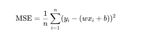
线性回归是机器学习中的常见算法,前些日子一直在看相关的数学知识,这次决定在AI的帮助下,用python实现一次线性回归算法。这里用均方误差公式函数配合梯度下降法,试图拿下这个东西。
线性回归你的目的是找到一个形似y=wx+b的公式,w是权重,b是偏置。
第一步,先提供一个基础模板
1
2
3
4
5
6
7
| import numpy as np
import matplotlib.pyplot as plt
np.random.seed(1)
x=np.random.rand(100,1)
y=4*x+3+np.random.randn(100,1)
|
第二步,我们写一个类,实现线性回归
1
2
3
4
5
6
7
8
9
10
11
12
13
14
15
16
17
18
19
20
21
22
23
24
25
26
| class LinearRegression:
def __init__(self, learning_rate=0.01, iterations=1000):
self.learning_rate = learning_rate
self.iterations = iterations
self.w = 0
self.b = 0
def fit(self, x, y):
m = len(x)
for _ in range(0, self.iterations):
y_pred = self.predict(x)
error = y - y_pred
dw = (2 / m) * np.dot(x.T, error)
db = (2 / m) * np.sum(error)
self.w -= self.learning_rate * dw
self.b -= self.learning_rate * db
def predict(self, x):
return self.w * x + self.b
|
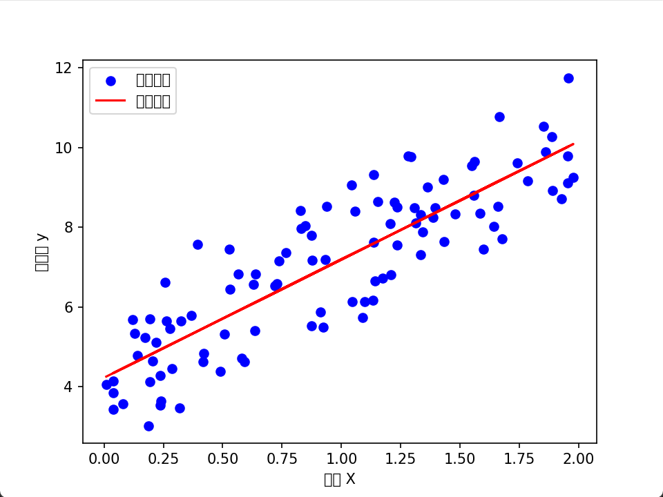
最后一步,让数据可视化
1
2
3
4
5
6
7
|
plt.scatter(X, y, color='blue', label='真实数据')
plt.plot(X, model.predict(X), color='red', label='拟合直线')
plt.xlabel('特征 X')
plt.ylabel('目标值 y')
plt.legend()
plt.show()
|
借助AI,理清楚思路,首先梯度的计算是借助一个循环进行的,循环次数是我们自己设定。求偏导就是得到的参数,
或者用已有的python库:
1
2
3
4
5
6
7
8
9
10
11
12
13
14
15
16
17
18
19
20
21
22
23
24
25
26
27
28
29
30
| from sklearn.linear_model import LinearRegression
from sklearn.metrics import mean_squared_error, r2_score
model = LinearRegression()
model.fit(x, y)
w_sklearn = model.coef_[0][0]
b_sklearn = model.intercept_[0]
print(f"sklearn实现的权重w: {w_sklearn:.4f}, 偏置b: {b_sklearn:.4f}")
y_pred_sklearn = model.predict(x)
mse = mean_squared_error(y, y_pred_sklearn)
r2 = r2_score(y, y_pred_sklearn)
print(f"均方误差(MSE): {mse:.4f}")
print(f"决定系数(R²): {r2:.4f}")
plt.scatter(x, y, label='真实数据', alpha=0.6)
plt.plot(x, y_pred_sklearn, color='green', label=f'拟合直线: y={w_sklearn:.2f}x+{b_sklearn:.2f}')
plt.xlabel('x')
plt.ylabel('y')
plt.legend()
plt.title('sklearn实现线性回归')
plt.show()
|
结果如图所示